Intuitive understanding of backpropogation
Backpropagation is one of the most skipped or overlooked algorithms in the deep learning space. It involves calculus, gradient tracking, chain rule, and a bunch of stuff that can look scary at first.
But at its core, backpropagation is simple.
In this blog, I will try to decode backpropagation intuitively.
Let’s see how it goes.
I will be explaining this in 3 parts:
- FeedForward Algorithm
- Intuition + Maths
- Backpropagation Algorithm
FeedForward Algorithm
Imagine we have a car.
When we press the gas pedal, the car does not move just because we pressed the pedal directly. The gas pedal is connected to a full internal system. Pressing the pedal triggers several internal mechanisms, and finally the output we desire happens: the vehicle moves forward.

A neural network also works in a similar way during feedforward.
Input enters the network, passes through neurons, gets multiplied by weights, goes through activation functions, and finally produces an output.
Consider a neuron N1 with input value x and weight w1.
The output will be:
output_N1 = w1 * xThis output is then passed to the next neuron N2, which has its own weight w2.
So the output of N2 becomes:
output_N2 = output_N1 * w2Note: For simplicity, we are ignoring bias for now.
If we keep doing this for many neurons, like:
N1 -> N2 -> N3 -> ... -> N100The whole network is still just multiplying values in a linear fashion.
That means the network behaves like a simple linear function:
y = mxWhere:
yis the outputmis weightxis input
This is not enough for real-world problems.
Real-world data is messy and non-linear.
For example:
- Image classification
- Object detection
- Speech recognition
- Language translation
- Stock prediction
- Medical diagnosis
These problems cannot be solved well using only simple linear transformations.
To solve this, we use activation functions.
Activation functions introduce non-linearity into the network.
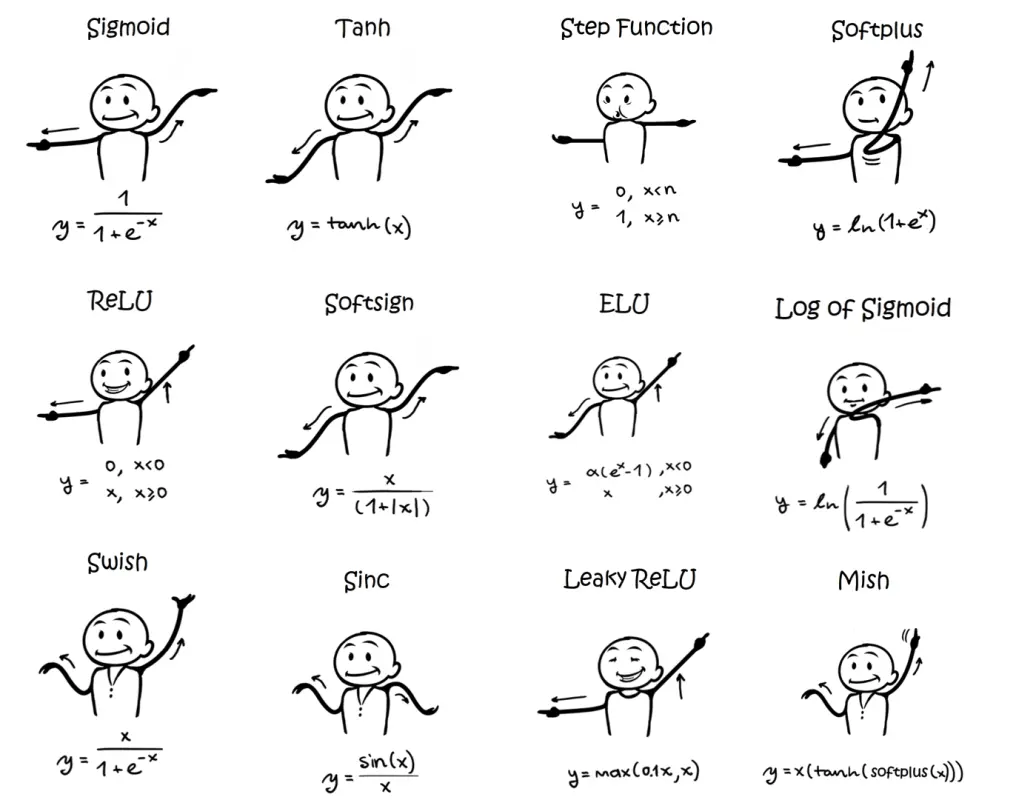
Some common activation functions are:
- ReLU
- Leaky ReLU
- Sigmoid
- Tanh
Mostly, ReLU is widely used in deep learning models.
Some activation functions:
Now the flow becomes:
Input -> weight multiplication -> activation function -> next neuronOr:
N1 -> output -> activation_function(output) -> input to N2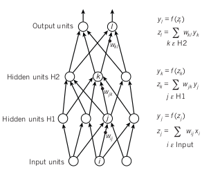
As shown in the image, input neurons get multiplied by weights and are passed to the next layer.
Note: When one neuron receives more than one input, we take the summation of all weighted inputs and then apply activation function on top of it.
For example:
z = w1x1 + w2x2 + w3x3 + b
a = activation(z)
Where:
zis the weighted sumais activated outputbis bias
Finally, the last layer gives us the prediction.
This prediction is compared with the actual label using a loss function.
That is where backpropagation enters.
Backpropagation Algorithm
A great analogy I heard once:
Imagine you are an intern in a company.
You do some task and send it to your manager. Your manager forwards it to the senior manager. Senior manager forwards it further. Eventually, the work reaches the CEO.
Now suppose the company suffers a loss.
CEO blames the senior manager.
Senior manager blames the manager.
Manager blames you.
You then correct your work based on the feedback and send it again.
That is pretty much how backpropagation works.
The loss function checks how bad the network performed.
Backpropagation then sends this error backward through the network and calculates how much each weight contributed to the error.
Then the weights are updated.
This process keeps repeating until the network learns better weights.
In theory, this is easy to understand.
But the maths makes it confusing.
Basic calculus is useful here, especially the chain rule.
Backpropagation, even by its name, tells us that it follows a backward direction.
Some basic shorthand we will use:
C: Cost/Loss functionσ: Activation functionŷ: Predictiony: Actual labelz: Weighted sum before activationa: Activated output
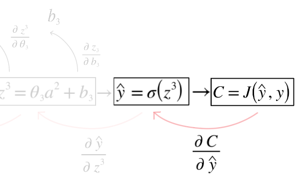
In the above image, we are taking partial differentiation of the cost function with respect to prediction ŷ.
But why?
Because we want to know:
How much did the prediction affect the final loss?The prediction did not appear magically.
It came from the final neuron.
Something like:
input -> weights -> weighted sum -> activation -> prediction -> lossSo when we ask:
How much did this weight contribute to the final error?We cannot answer it directly.
Because a weight affects neuron output.
Neuron output affects the next layer.
Next layer affects the prediction.
Prediction affects the loss.
So we use the chain rule.
That is the heart of backpropagation.
Intuition + Maths
Let’s take a very small neural network.
x -> w1 -> a1 -> w2 -> ŷ -> CWhere:
a1 = w1 * x
ŷ  = w2 * a1
C  = 1/2(ŷ - y)^2
Here:
xis inputyis actual answerŷis predicted answerCis cost/error
Now, if the cost is high, we want to know:
How should w1 and w2 change to reduce C?For w2, the derivative is:
∂C/∂w2 = ∂C/∂ŷ * ∂ŷ/∂w2For w1, the derivative is:
∂C/∂w1 = ∂C/∂ŷ * ∂ŷ/∂a1 * ∂a1/∂w1This is backpropagation.
We are walking backward from cost to weights and asking:
How much did this part affect the final error?Now let’s include activation function.
z1 = w1x + b1
a1 = σ(z1)

z2 = w2a1 + b2
ŷ  = σ(z2)
Then derivative for final layer weight becomes:
∂C/∂w2 = ∂C/∂ŷ * ∂ŷ/∂z2 * ∂z2/∂w2Which means:
error at output
x activation derivative
x previous layer output
So for output layer:
∂C/∂w = (ŷ - y) * σ'(z) * a_previousThis tells us how much the weight should change.
What is Gradient?
Gradient is just direction.
It tells us which way we should move the weight to reduce loss.
If gradient is positive, decreasing the weight may reduce the loss.
If gradient is negative, increasing the weight may reduce the loss.
That is why the weight update rule looks like this:
w = w - learning_rate * gradientThe learning_rate controls how big the correction step should be.
If the learning rate is too small, learning will be slow.
If the learning rate is too large, the model may jump around and never settle properly.
So learning rate matters a lot.
Backpropagation Algorithm
At a high level, training a neural network looks like this:
1. Initialize weights randomly

2. FeedForward:
   - Pass input through the network
   - Calculate prediction

3. Calculate Loss:
   - Compare prediction with actual answer

4. Backpropagation:
   - Start from loss
   - Calculate gradients layer by layer backward

5. Update weights:
   - weight = weight - learning_rate * gradient

6. Repeat many times
More technically:
For every layer:

Forward:
z = wx + b
a = activation(z)

Backward:
Find ∂C/∂w and ∂C/∂b using chain rule

Update:
w = w - η * ∂C/∂w
b = b - η * ∂C/∂b
Where η is the learning rate.
Small Numerical Example
Assume:
x = 2
w1 = 3
w2 = 4
y = 30
Forward pass:
a1 = x * w1 = 2 * 3 = 6
ŷ  = a1 * w2 = 6 * 4 = 24
Actual value is 30.
Prediction is 24.
So error is:
ŷ - y = 24 - 30 = -6The model predicted too low.
Now gradients will tell the model:
Increase weights in a direction that increases prediction.For w2:
∂C/∂w2 = (ŷ - y) * a1
       = -6 * 6
       = -36
For w1:
∂C/∂w1 = (ŷ - y) * w2 * x
       = -6 * 4 * 2
       = -48
Assume learning rate is 0.01.
Update:
w2 = 4 - 0.01 * (-36)
w2 = 4.36
w1 = 3 - 0.01 * (-48)
w1 = 3.48Both weights increased.
Why?
Because prediction was lower than the actual value.
So the model needs to push output upward.
This is learning.
Why Backpropagation Feels Confusing
Backpropagation feels confusing because it is usually taught from equations first.
But the real idea is simple:
Prediction was wrong.
Find who contributed to the mistake.
Change them slightly.
Repeat.
Every weight gets a blame score.
That blame score is called gradient.
Backpropagation is just an efficient way to calculate this blame score for every weight in the network.
Final Intuition
Feedforward is like:
Input goes forward and creates prediction.Backpropagation is like:
Error goes backward and corrects weights.Forward pass answers:
What does the model predict?Backward pass answers:
How should the model change?And training is this loop again and again:
predict -> compare -> blame -> correctThat’s pretty much backpropagation.
The maths may look scary, but the intuition is not.
It is just the chain rule applied repeatedly across layers.
Conclusion
Backpropagation is not magic.
It is simply a systematic way of calculating how much each weight contributed to the final error.
Once we know that, we update the weights in the opposite direction of the error.
That is how neural networks learn.
The whole deep learning training process can be summarized as:
Forward pass gives prediction.
Loss function gives mistake.
Backpropagation gives correction.
Optimizer applies correction.
And this loop, repeated thousands or millions of times, slowly turns random weights into a useful model.
~ Until next time, Hitesh